Eigenvector Method

Eigenvalues are a unique collection of scalar values linked to a set of linear equations, most commonly in matrix equations. Eigenvalues are also called characteristic roots or latent roots. After applying linear transformations, it is a non-zero vector that its scalar factor can only alter. An eigenvalue is the scale factor that correlates to the eigenvectors. The direction of the eigenvector never changes if a body rotates or twists along its axis. The eigenvectors are a type of vector which is associated with a set of linear equations. Eigenvectors are used to make linear transformation understandable.

Eigenvector method

Within the evaluation of linear transformations, eigenvalues and eigenvectors play a significant role. The prefix eigen- comes from the German word eigen, which means ‘property’, ‘function’, or ‘own’. Eigenvalues and eigenvectors are used in a wide range of applications, including balance evaluation, vibration evaluation, atomic orbitals, facial recognition, and matrix diagonalization. Eigenvalues and eigenvectors were initially used to observe predominant axes of the rotational motion of rigid bodies.

The eigenvalue is a non-zero vector that can be changed at most by its scalar factor after the application of linear transformations.

An eigenvector v of a linear transformation is what it sounds like. T is a non-zero vector that no longer alternates course while T is applied to it. Applying T to the eigenvectors only scales the eigenvector by the scalar value ,

called an eigenvalue. Because the equation can be written, this circumstance can be written.

The eigenvalue equation is also known as the eigenequation. can be any scalar in general. 

Practicing the eigenvector method

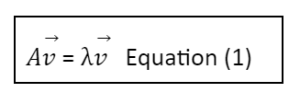
The eigenvector V of a matrix A is the vector for which the following holds in general:

where is a scalar value known as the eigenvalue. In this way, the linear transformation A on vector V is completely defined by the use of.

Equation (1) can be rewritten as follows:

I is the identity matrix that has the same dimensions as A.

If V isn’t always the null-vector, however, equation (2) can be best stated if A-I isn’t always invertible. If a rectangular matrix isn’t always convertible, its determinant must be the same as zero. As a result, to find the eigenvectors of A, we must first solve the following equation:

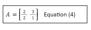
Using fixing equations, we may determine the eigenvectors and eigenvalues of a matrix A in the following sections (3). In this case, matrix A is described using the following formula:

Finding eigenvalues

Eigenvalues are calculated by multiplying the eigenvalues by the number of eigenvalues.

To determine the eigenvalues for this case, we substitute A in equation (3) with equation (4):

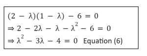
When you calculate the determinant, you get:

We use the discriminant to solve this quadratic equation in :

Because the discriminant is exactly positive, there are exceptional values for:

The two eigenvalues 1 and 2 have now been determined. It’s worth noting that a rectangular matrices of length NN usually have exactly N eigenvalues, each with its eigenvector. The eigenvalue determines the eigenvector’s scale.

The first eigenvector is calculated.

We can now get the eigenvectors by putting the eigenvalues from equation (7) into equation (1).

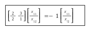
Start with eigenvalue 1 to find the appropriate first eigenvector:

We may write it in its equivalent form because it is absolutely the matrix notation for a device of equations:

As a result, if you solve the primary equation as a function of x12  you’ll get:

Because an eigenvector indicates a direction while the associated eigenvalue conveys magnitude, all of its scalar multiples are vectors that can be parallel to it and are hence similar. If might normalize the vectors, they can all be equal. So, rather than fixing the above equations, we can freely choose a real value for x11 and x12, and determine the opposite via equation (9).

For this example, we choose X12 = 1 at random so that X11=-1. As a result, the eigenvector with the eigenvalue = -1 is:

The second eigenvector is calculated.

The calculations for the second eigenvector are identical to those for the first; we now substitute eigenvalue Y2 = four into equation (1), yielding:

The equation can be written as:

Solving the basic equation as a property of X21 yields the following:

We then choose x21 = 2 at random and look for x22 = 3. As a result, the eigenvector for the eigenvalue 2 = 4 is: