Profile
 Settings
 Refer your friends
 Sign out


Lagrange’s equation is imperative in mechanics, used for determining various properties of mechanical systems such as motion. In 1788, Joseph-Louis Lagrange proposed the equation. For “simple systems”, Newton’s equations are well known, but when it comes to finding the mechanical properties of “real systems,” Newton’s equations are difficult to solve as the complexity increases. The equations of Lagrange are used in such situations since they allow for some limitations to be avoided, and are also presented in a standard form. Later, Lagrange’s equation became known as ‘Analytical Mechanics’. Let’s take a closer look at Lagrange’s equation in this article.
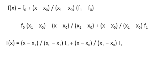
![]() To write the Lagrange interpolation equation, use simplified notations simplified notations f0 = f(x0), f1 = f(x1):
To write the Lagrange interpolation equation, use simplified notations simplified notations f0 = f(x0), f1 = f(x1):
![]()
![]() If you collect the terms for f0, f1, and f2, and then do some tedious algebraic trickery, you can write the Lagrange interpolation second-order formula as
If you collect the terms for f0, f1, and f2, and then do some tedious algebraic trickery, you can write the Lagrange interpolation second-order formula as
![]()
![]() In order for each term of *j (x) to be equal to 1, (a) *j (xi) must be 0, and (b) *j (xj) must be 1. Since the above property ensures that f(xj) = fj, no other samples (fi, i = j) are eligible to participate.
In order for each term of *j (x) to be equal to 1, (a) *j (xi) must be 0, and (b) *j (xj) must be 1. Since the above property ensures that f(xj) = fj, no other samples (fi, i = j) are eligible to participate.
What is Lagrange’s equation?
When a solid mechanics problem is analyzed, Lagrange’s equation is used to determine the solution, but rather than using forces, it uses the energy in the system. The acceleration is not needed to solve the problem, but it must be solved for the inertial velocities as discussed earlier. In general, the Lagrange equation is written as follows: L = T – V L is a notation for Lagrange’s equation T is the kinetic energy of the system V is the potential energy of the system A system’s potential energy is determined by the coordinates of its particles, while its kinetic energy generally depends on its velocities. An individual system’s potential energy and kinetic energy can be expressed numerically as V = V (x1, y1 , z1 , x2 , y2 , z2 , . . . ) and T = T (x’1 , y’1 , z’1 , x’2 , y’2 , z’2 , . . .) respectively. This Lagrangian L is dependent upon all six dynamic variables. For conservative systems Lagrange’s equation is expressed as: d/dt (მL/მ’qi) – მL/მqi = 0 The equations of motion of the system are described by differential equations resulting from the above equation.Lagrange’s Interpolation Formula
By using Lagrange’s interpolation formula, a polynomial known as the Lagrange polynomial can be obtained. Consider the case when there are n numbers of distinct real values (x1, x2, …, xn) and n numbers of real values (y1, y2, …, yn) which may or may not be distinct. For every i ∈ [1, 2, …, n], there exists a unique real coefficient polynomial P which satisfies P (xi) = yi, such that the Lagrange’s polynomial is less than n. This polynomial takes a particular value at random points. Many Lagrange interpolation formula solved examples can be found on the internet.Lagrange First Order Interpolation Formula
In Lagrange interpolation formula of first order, it is given that,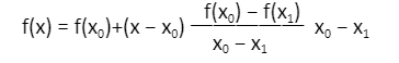 To write the Lagrange interpolation equation, use simplified notations simplified notations f0 = f(x0), f1 = f(x1):
Lagrange Second-Order Interpolation Formula
In Lagrange interpolation formula of second order, it is given that: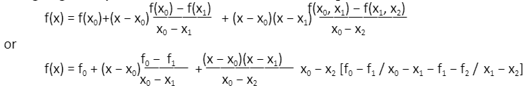 If you collect the terms for f0, f1, and f2, and then do some tedious algebraic trickery, you can write the Lagrange interpolation second-order formula as
Lagrange N-th Order Interpolation Formula
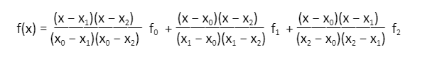
Lagrange Interpolation formula of N-th order can be expressed in the form of: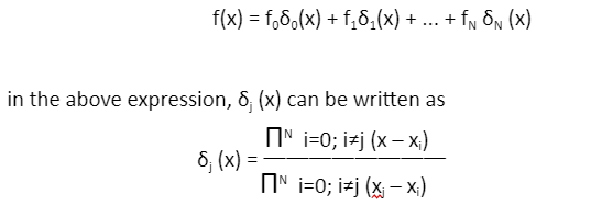 In order for each term of *j (x) to be equal to 1, (a) *j (xi) must be 0, and (b) *j (xj) must be 1. Since the above property ensures that f(xj) = fj, no other samples (fi, i = j) are eligible to participate.