Graphs of Linear Equations

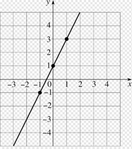
A linear equation is a two-variable equation with a line as the graph. A set of points in the coordinate plane that are all solutions to the equation make up the graph of a linear equation. If all variables are real values, the equation can be graphed by drawing enough points to notice a pattern and connecting the points to include them.

You must have at least two points to graph a linear equation, though it is highly advisable to include additional. Try to incorporate both positive and negative numbers, as well as zero, when choosing your points.

After understanding the definition of the linear equation!

Linear Equation Formula

A linear equation is expressed using the linear equation formula. This can be accomplished in a variety of ways. For example, a linear equation can be written in standard form, slope-intercept form, or point-slope form. Let’s look at the usual form of a linear equation and see how it is written. We can see that it fluctuates depending on the number of variables, and it is important to remember that all variables in the equation should have the highest (and only) degree of 1.

y= MX + B

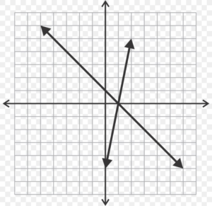
Graph a system of linear equations

We will look at graphing of linear equations and inequalities in two variables in this part. We will begin by practising graphing two equations on the same axes, and then we will go over the many aspects to consider when graphing two linear inequalities on the same axes. Use the same methods you used to graph single linear equations to graph a system of linear equations. To graph both lines on the same set of axes, we can utilise tables of values, slope and y-intercept, or x– and y-intercepts.

Take, for example, the two-variable system of linear equations below.

2x+y is equal to−8 and x−y is equal to −1

First, solve for y in 2x+y=−8

2x+y is equal to−8

y is equal to −2x−8

Second, solve for y in x−y is equal to −1

x−y is equal to −1

y is equal to x+1

The system is now written as

y is equal to −2x−8

y is equal to x+1

Graphing a Linear Function Using y-intercept and Slope

Instead of charting dots, another technique to graph linear functions is to use certain properties of the function. The first characteristic is the y-intercept or point where the input value is zero. Set x=0x=0 in the equation to determine the y-intercept.

Another aspect of the linear function is its slope, which is a measure of how steep it is. Remember that the slope is the function’s rate of change. The ratio of the change in outputs to the change in inputs is the slope of a linear function. To calculate the slope, multiply the vertical difference, or ascent, between any two places by the horizontal difference, or run. A linear function’s slope will be the same at any two places. In Linear Functions, we encountered both the y-intercept and the slope.

Use a graph to classify solutions to systems.

Remember that linear equation graphs as a line, indicating that every point on the line is a solution to the linear equation. There are a limitless amount of possibilities. As we learned in the last section, if a system of linear equations intersects at one point, that point represents the system’s solution. What if the lines never cross, as they do when parallel lines are drawn? What words would you use to characterise the solutions to such a system? In this section, we will look at the three possible outputs of a system of linear equations solution.

Graphing a Linear Function Using Transformations

Transformations of the identity function f(x) =x are another option for charting. A shift up, down, left, or right can modify a function. A reflection, stretch, or compression can also be used to change a function.

Vertical Stretch or Compression

The m acts as the vertical stretch or compression of the identity function in equation f(x)=mx. When m is negative, the graph also has a vertical reflection. Multiplying f(x)=xf(x)=x by m stretches the graph of f by a factor of m units if m>1 and compresses the graph of f by a factor of m units if 0<m<1. The steeper the slope, the greater the absolute value of m.

Tips on Linear Equations

• The solution or root of a linear equation is the value of the variable that makes the equation true

• Adding, subtracting, multiplying, or dividing the same integer into both sides of a linear equation does not affect the solution

• The graph of a one- or two-variable linear equation is always a straight line

Conclusion

That’s a wrap to the crucial aspects of linear functions and graphing of linear equations with graphs and illustrations! 

There is no denying that every application of mathematics has systems of equations. They are useful for figuring out and articulating how behaviours and processes are linked. It is uncommon to see a traffic flow pattern solely influenced by the weather. You might have learned about creating graphs using transformations, y-intercept and slopes, linear equations, etc.