Calculating Electric Fields of Charge Distributions

Microscopically, the electric charge is quantised. It isn’t easy to look at individual charges in charged bodies when dealing with their electric fields. As a result, the charge is thought to be spread continuously, and its discrete nature is ignored. The electric field resulting from such continuous charge distributions is calculated using the calculus approach.

There is no such thing as a “really” continuous charge distribution because the charge is quantised. In most practical circumstances, however, the overall charge forming the field consists of many discrete charges. This means we may safely disregard its discrete nature and treat it as continuous. We apply a similar approximation when dealing with a bucket of water as a continuous fluid rather than a collection of water molecules.

Electric Fields 

We can use one of the charges as a “given” and the other as a “test particle” whenever we have two charges. We can move the test particle around in space and measure the amount of force it experiences at different points. There is a magnitude and a direction to the force. Imagine a small arrow drawn at each point in space. The arrow’s length is proportional to the force’s size, and the arrow’s direction matches the forces. We would have filled all of the space with little arrows when we’re through. The entire collection represents a field.

A field is a set of values that describe how a quantity is affected by its location or by both location and time. We need to employ a test particle with a one-unit positive charge to make it match the formal description. Since the electric charge is measured in coulombs, we will use a test charge of +1 coulomb to do this imaginary test and get the right electric field. To summarise, an electric field is a map representing the force that a +1 coulomb test charge would feel at any given position.

We can observe that the size and direction of these small arrows gradually change if we draw them all. We can create continuous lines that follow the arrows in a type of connect-the-dots game. They’re called Electric field lines. These arrows will point either in the direction of the provided charge (if it’s negative) or away from it (if it’s positive). The square of the distance between the two charges determines the size of the arrows. The size will be reduced by a factor of four if we double the separation. “Inverse-square law effects” describe how things act in this way.

Discrete Charge Distribution

What if we had two charged objects and the same +1 coulomb test charge? Both of the other charges would now exert force on the test charge. Each component would still be pointing toward or away from the surface charge density that created it, but adding the two forces together may result in a total force pointing in a different direction. The sum of the electric fields formed by the two charges will be the electric field created by each one. This method works for any number of charges (a thousand, a million, even a billion). We can add the components together and draw an arrow based on the sum.

We’ve assumed that all of the charges are at precise small places in space up to this point. Because we wish to find the field values at specific positions in space, the test charge must always be so. A discrete charge distribution is one in which the specified charges are also at specific places. Discrete, in this context, means ‘At specific positions’.

By referring to the overall volume of the distribution as V, the total volume of distribution, and DV, the incremental charge volume, which is defined as the charge point. The Greek letter Rho is used to represent this quantity, which is equal to the total distribution charge divided by the total distribution volume.

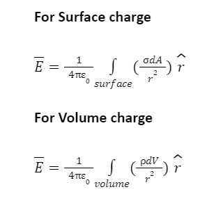
Electric field for various charge distribution is calculated by following formulas

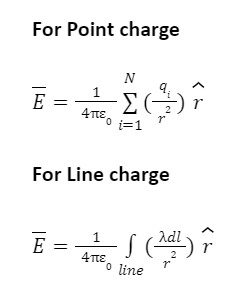
Where

q = charge (Cb)

Λ = charge per unit length (linear charge density); units are coulombs per meter (C/m)

σ = charge per unit area (surface charge density); units are coulombs per square meter (C/m2)

የ = charge per unit volume (volume charge density); units are coulombs per cubic meter (C/m3)

Conclusion

So far, the charge distributions we’ve seen have been discrete, consisting of single point particles. On the other hand, a continuous charge distribution has at least one nonzero dimension. We can generalise the definition of the electric field if the charge distribution is continuous rather than discrete. We divide the charge into microscopic fractions and treat each fraction as a point charge.