Mean value theorem

The mean value theorem follows the rules and properties of the real numbers and is an essential calculus theorem. The theorem is a result of empirical work done in Kerala, India. The concept was proposed in the 14th century by a mathematician named Parmeshwara Nambudiri. To help students understand the mean value theorem, most mathematics teachers teach Rolle’s theorem first. French mathematician Michel Rolle developed Rolle’s theorem in the 17th century, and it is a less complicated version of the mean value theorem. Currently, the mean value theorem in use is the one proposed by Augustin Cauchy and it is more generalized than its predecessors.

What is the Mean value theorem?

The mean value theorem is defined mathematically as the existence of a point c in the interval (a, b) for which the function (f) is continuous on the closed interval [a, b] and differential on the open interval (a, b) such that f’(x) equals the function’s average rate of change over a period (a, b). To put it simply, a curve passes through two points for one point on the curve under the mean value theorem for which the tangent and secant are parallel.

It can be shown that the mean value theorem for a function f (x) is: [a, b] → R, across an interval, then, there is a number c such that a < c < b. In this case f’ (c) is expressed as:

As seen in the expression above, there is a point c on the interval f(x) for which the function is continuous at the closed interval [a, b] and differentiable at the open interval (a, b). In other words, this shows that the tangent at point c is parallel to the secant passing through the two given points (a, f(a)), (b, f(b)). The above formula is also used to calculate the value of c in the integral mean value theorem.

Proving the Mean value theorem

In what we have seen so far, the mean value theorem states that there exists at least one point or point c in the interval (a, b) for which a function (f) is continuous on the closed interval (a, b) and differentiable on the open interval (a, b), such that f(c) represents the average rate of change of the function over [a,b], and that it is parallel to the secant line over [a,b].

According to Rolle’s theorem, suppose that f(a) = f(b) for a function (f) continuous over [a,b], differentiable over (a, b). In such a case, c exists where a < c < b and f’ (c) = 0. A function must level itself and will continue indefinitely after the first point only if it has a local maximum or minimum. This is because it can be determined whether the function increases or decreases after the first point. Thus, if the function, after an interval, returns to the same value, neither of the options can continue.

Proof:

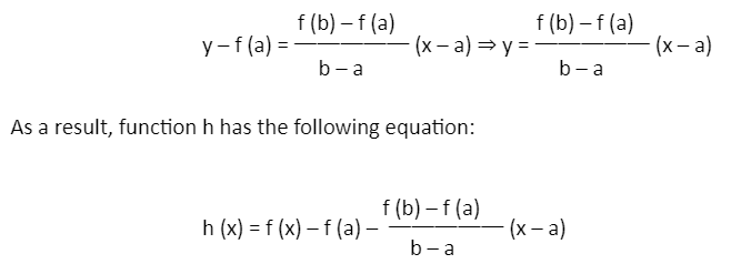
We will derive and prove the mean value theorem calculator. let h represent the difference between the function f and the line that passes through the points (a, f (a)) and (b, f (b)). Hence, the equation of the line can be expressed as:

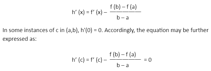
As a result, function h has the following equation:

In this way, Rolle’s theorem is used to prove the mean value theorem.

Conclusion

The mean value theorem demonstrates a correlation between a function’s behaviour and its derivative’s behaviour In conjunction with Rolle’s theorem and some mean value theorem examples, we can better understand the concepts of these theorems and gain a deeper understanding of how they work. The two theorems share a similarity regarding how they define function f (x) as being continuous over an open interval while being differentiable at the other. In the mean value theorem f (a) ≠ f (b) because the points are distinct and in Rolle’s theorem, the points are defined in such a way that f (a) = f (b).