Definition of mean value theorem
The mean value theorem is a key theorem in calculus. In the 14th century, Parmeshwara, a mathematician from the state of Kerala established the oldest version of the mean value theorem. In the 17th century, Rolle presented a simpler model of this theorem. This theorem was established for polynomials and was not to be considered in calculus. The latest iteration of the mean value theorem was presented by Augustin Louis Cauchy in 1823.
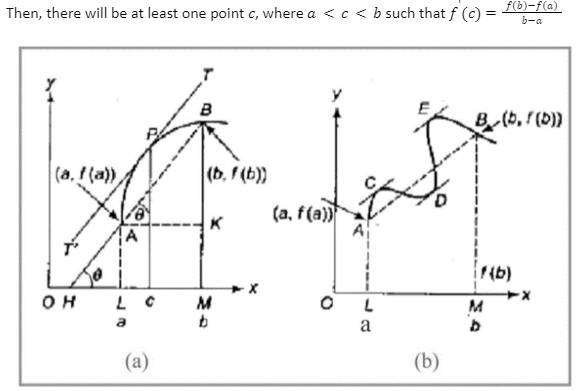
According to the mean value theorem, there is one point on a curve that runs between two points in which the tangent is parallel to the secant that runs between the two points. Rolle’s theorem is based on this mean value theorem. Here, we shall discuss Rolle’s Theorem and Lagrange’s mean value theorem. What are these theorems, the statements, the conditions, how to use them to solve problems will be covered in this concept.
Rolle’s theorem
Let f be a real-valued function referred to as the closed interval a,b such that
- It is continuous in closed interval represented as [a, b]
- It is differentiable in open interval represented as a, b and
- fa=fb, then there exist at least real number ‘c’∈a, b such thatf’c=0.
Geometrical Meaning:
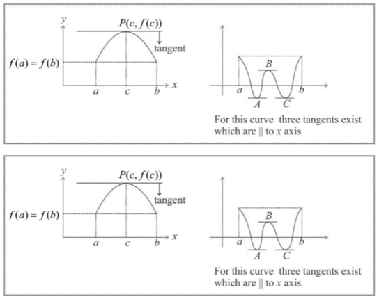
If fx be a real-valued function defined on a, b such that y=f(x) is continuous curve between points Aa, f(a), Bb,fb, there exists a unique tangent at every point on the curve y=fx between points A and B. Also, the ordinate points at the end of interval a,b are equal. There exists at least one point c, f(c) between A & B on the curve where tangents are parallel to x-axis.

Lagrange’s Mean Value Theorem
If a function of mean value theorem fx is
(i) Continuous in the close interval a, b, i.e., continuous at each point in the interval a,b
(Ii) Differentiable in the open interval a,b, i.e., differentiable at each point in the interval a,b

Proof of mean value theorem
To prove the mean value theorem, the function h(x) = f(x) – g(x) can be considered. Here, g(x) is referred to as the function which represents the secant line denoted as AB. Here, Rolle’s theorem is applied to the continuous function denoted as h(x), proving that the point c in (a, b) co-exists in a way that h'(c) = 0. The given equation will appear as the result of the mean value theorem.
Let g(x) be the secant line to f(x) passing through (a, f(a)) and (b, f(b)). We know that the equation of the secant line is y-y1 = m (x- x1).
y – f(a) = {f(b) – f(a)}/(b-a) . (x – a)
or y = f(a)+ {f(b) – f(a)}/(b-a) . (x – a)
Imagine h is the function that defines the difference between the above line and any function f.
Therefore, h(x) = f(x) – f(a) – {f(b)-f(a)}/(b-a) . (x – a)
When applying the Rolle’s theorem, we have
h(a)=0 and h(b)=0
h'(x) = f'(x) – {f(b)-f(a)}/(b-a)
Or f(b) – f(a) = f'(x) (b – a). Hence proved
Differences between mean value theorem and Rolle’s theorem
The distinction between Rolle’s theorem and the mean value theorem aids in comprehending these two theorems. Both these theorems speak about the f(x) as an ongoing function in and around the interval [a, b] and also the differentiable function in and around the interval [a, b] . In the mean value theorem, both these locations (a, f(a)), (b, f(b)) are different. In comparison, the points in Rolle’s theorem are expressed as f(a) = f (b).
Conclusion
In the 14th century, Parmeshwara, a mathematician from the state of Kerala established the oldest version of the mean value theorem. The latest iteration of the Mean Value Theorem was presented by Augustin Louis Cauchy in 1823. The mean value theorem is closely related to Rolle’s theorem, which we discussed here. Both the theorems have significant differences such as, in the examples of mean value theorem, both these locations (a, f(a)), (b, f(b)) are different from one another. However, in the case of Rolle’s theorem, these locations are expressed as f(a) = f(b).
 Profile
 Settings
 Refer your friends
 Sign out


