Bernoulli’s theorem is a statement in fluid mechanics that relates the pressure and velocity of a flowing fluid. It is called after Daniel Bernoulli, who broadcasted it in his book Hydrodynamica in 1738. The theorem states that for an inviscid flow (a flow where the viscosity of the fluid can be ignored), the sum of the pressure and kinetic energy per unit volume is constant. In other words, as the velocity of a fluid increases, its pressure decreases. This theorem has many applications in physics and engineering, and we will discuss some of them in this blog post.
In liquid dynamics, Bernoulli’s theorem states that an upsurge in the pace of a fluid occurs simultaneously with a decrease in pressure or a reduction in the potential energy of the fluid. The theorem is prescribed after Daniel Bernoulli who printed it in his book Hydrodynamica in 1738.
Bernoulli theorem has a lot of use in fluid mechanics. It can be used to derive the Bernoulli equation which is a very important equation in fluid mechanics. Here are some examples of applications of Bernoulli’s theorem:
-working of aeroplane:
An aeroplane works on the principle of Bernoulli’s theorem. When an aeroplane flies, the wings create a low-pressure area above them. This low-pressure area sucks the air from below the wings and creates lift.
-working of a venturi:
A venturi is a device that is used to measure the flow rate of a fluid. It works on the principle of Bernoulli’s theorem. The fluid is accelerated as it passes through a narrow constriction in the venturi. This causes a decrease in pressure which can be measured.
A pitot tube is used to measure the rate of a fluid. It works on the principle of Bernoulli’s theorem. The fluid is accelerated as it passes through a narrow constriction in the pitot tube. This causes a decrease in pressure which can be measured.
An atomiser is a device that is used to spray a liquid in the form of fine droplets. It works on the principle of Bernoulli’s theorem. The liquid is accelerated as it passes through a narrow constriction in the atomiser. This causes a decrease in pressure which vaporises the liquid and breaks it up into fine droplets.
So these are some examples of applications of Bernoulli’s theorem.
Bernoulli’s equation can be derived from the conservation of energy equation. If we consider a control volume that is moving with the fluid, Bernoulli’s equation states that the sum of all forms of energy within the control volume must remain constant.
Here is the bernoulli equation:
p+1/2V2+gh=constant
where:
P is the pressure
is the density
V is the velocity
H is the elevation
G is the gravitational accelarartion
So this was all about the derivation of Bernoulli’s theorem.
Bernoulli’s equation has certain limitations:
-It is a statement of energy conservation and as such, it cannot be applied to open systems.
-It is only strictly valid for inviscid, incompressible flow. However, it can be applied to viscous flow if the fluid speed is small enough and the fluid density is constant.
-It is only valid for steady flow. However, it can be applied to unsteady flow if the fluid speed is small enough and the fluid density is constant.
-It cannot be applied to flow with a significant change in elevation (i.e. large height difference between the two points where the pressure is measured).
-It cannot be applied to flow with significant curvature (i.e. the fluid path between the two points where the pressure is measured is not straight).
-It cannot be applied to flow with significant friction (i.e. the fluid is moving through a pipe or other constriction).
-It cannot be applied to flow with significant heat transfer (i.e. the fluid temperature is changing).
-It cannot be applied to flow with significant electrical effects (i.e. the fluid is conducting electricity).
-It cannot be applied to flow with significant magnetic effects (i.e. the fluid is moving through a magnet).
-It cannot be applied to nuclear reactions (i.e. the fluid is radioactive).
-It cannot be applied to gravitational effects (i.e. the fluid is under the influence of gravity).
-It cannot be applied to flow in a vacuum (i.e. there is no fluid).
So there you have it! Three examples of Bernoulli’s Theorem in action. Of course, this is just a tiny sampling of all the places you’ll find Bernoulli’s Theorem at work. This principle is truly ubiquitous in fluid mechanics! The application of the Bernoulli theorem is not just limited to ideal fluids but also non-ideal fluids. Bernoulli’s theorem can be applied to derive the Bernoulli equation which is widely used in fluid mechanics. We hope you enjoyed this quick tour of Bernoulli’s Theorem. Hopefully, this article has given you a better understanding of how and where Bernoulli’s Theorem crops up in the world around us. Thanks for reading!
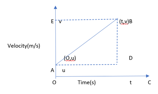
The body has initial velocity u (measured by line OA). The object is uniformly accelerated motion (the slope is a straight line inclined to the X-axis). The acceleration value is a. The object reaches its final velocity v (measured by line OE). The time duration of this motion is t seconds. Let the distance travelled covered by the object in time t be s.
u=OA, v=BC, t=OC
The slope of the velocity-time graph=acceleration of the moving object
a=(yb-ya)/(xb-xa)
a=(v-u)/(t-0)
at=v-u
On rearranging,
v-u=at OR
v=u+at (first equation of motion)
s=area of OABC
=area of rectangle OADC+area of triangle ABD
=(length*breadth)+½*base*height
+OA*OC+½ *AD*BD _______________(1)
From the graph, we know:
AD=OC=t
BD=EA=OE=OA=v-u
Substituting in equation (1):
s=(u*t)+½ *t*(v-u)
Using at=v-u:
s=ut+½ *t*at OR
s=ut+½ at2 (Second equation of motion)
s=½*(sum of parallel sides)*height
=½(OA+BC)*OC
=½(u+v)*t
Using t=(v-u)/a:
s=½(u+v)*(v-u)/a
=½(v+u)(v-u)
2as =(v2-u2)
v2-u2=2as (Third equation of motion)
The equations of motion are only applicable, however, in cases, where:
Motion can be of numerous types. It is not that everything moves in the same fashion. For instance, it can be in a straight line, or in a circle. Therefore, the motion has been classified into several different types. The most basic classification of motion consists of four main types of motion. These are:
The following are some examples of motion involving acceleration (positive or negative):
An object is said to be in accelerated motion if its velocity changes throughout the course of its motion. It is the rate of change of motion per unit time. Acceleration can be either positive or negative. If the acceleration is negative, the motion is also known as retarded motion. In cases pertaining to rectilinear motion with uniform acceleration, the components of motion can be predicted by using the equations of motion. There are three equations of motion. The slope of the velocity-time graph gives acceleration while the area under the velocity-time graph represents the total distance.


 Profile
 Settings
 Refer your friends
 Sign out