The Discrete probability distribution and the continuous probability distribution are two types of probability distributions that define discrete and continuous random variables respectively. A probability distribution can be defined as a function that describes all possible values of a given random variable as well as its associated probabilities.

Discrete Probability Distribution Definition

The discrete probability distribution can be defined as the probability distribution giving the probability that a discrete random variable will have a specific value. Such distribution will represent data that has a finite countable number of outcomes. There are two conditions that a discrete probability distribution should satisfy. They are given as follows:

• 0 ≤ P(X = x) ≤ 1. This states that the probability of a discrete random variable, X, taking on an exact value, x, lies between 0 and 1.
• ∑P(X = x) =1. The sum of all probabilities should be equal to 1.

Discrete Probability Distribution Example

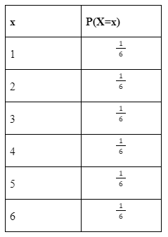
Suppose a fair dice is rolled and the discrete probability distribution is created. The possible outcomes are {1, 2, 3, 4, 5, 6}. Therefore, the total number of outcomes will be 6. Every number has an equal chance of coming up. This means that the probability of getting any one number facing up is 1 / 6. Using the given data the discrete probability distribution table for the dice roll can be given as follows:

Discrete Probability Distribution Types

The discrete probability distribution is often used in a Monte Carlo simulation in order to find the probabilities. The commonly used types of discrete probability distributions are given below.

Bernoulli Distribution

The Bernoulli distribution is a type of discrete probability distribution where the random variable can either be equal to 0 or be equal to 1. The probability of getting success is p and getting a failure is 1 – p. The pmf is expressed as follows:

Binomial Distribution

The binomial distribution is a discrete probability distribution that results in the success probability in the n Bernoulli distribution. The probability of being successful is given by p. It is denoted as X ∼ Binomial (n, p). The pmf is given below:

Geometric Distribution

A geometric distribution is another type of discrete probability distribution that represents the probability of getting a number of successive failures till the first success is obtained. It is denoted X ∼ G(p). The formula for the pmf is given as:

P(X = x) = (1 – p)x p, where p is the success probability of the trial.

Poisson Distribution

The Poisson distribution is a discrete probability distribution that is mostly used in the field of finance. It gives the probability that a given number of events will take place within a fixed period of time. The notation is written as X ∼ Pois(λ), where λ>0λ>0. The pmf is given by the following formula:

Finding Discrete Probability Distribution

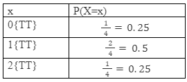
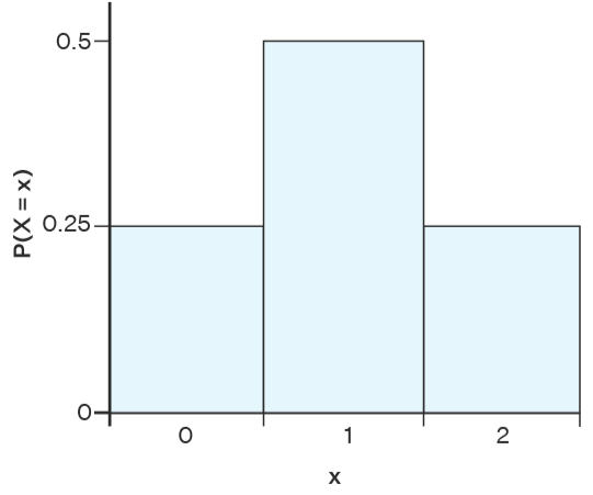
The discrete probability distribution can be represented either in the form of a table or with the help of a graph. To find a discrete probability distribution we need the probability mass function. In other words, to construct a discrete probability distribution, all the values of the discrete random variable and the probabilities associated with it are required. For example, a fair coin is tossed twice. The discrete probability distribution can be determined from the number of heads. The steps are given below:

• Step 1: Determine the sample space of the given experiment. When a fair coin is tossed twice the sample space would be {HH, HT, TH, TT}. Here, H denotes heads and T represents tails. Hence, the total number of outcomes is 4.
• Step 2: Define a discrete random variable, X. For the example let X be the number of heads observed.
• Step 3: Identifying the possible values. There will be  3 possible values of X. Those are 0 ( which means no head is observed), 1 ( which means exactly one head is observed), and 2 ( which means the coin lands on heads twice).
• Step 4: Now Calculate the probability associated with each outcome. In the example, the probability can be calculated by the formula, a number of favourable outcomes / total number of possible outcomes.
• Step 5: To get the discrete probability distribution to represent the probabilities and the corresponding outcomes in tabular form or in graphical form. This is expressed as given below:

A histogram will be used to represent a discrete probability distribution like in this graph

Conclusion

Here in this article, we have discussed the discrete probability distribution. We have discussed the discrete probability distribution with examples. The discrete probability distribution are of different types like Bernoulli’s distribution, binomial distribution, geometric distribution, and Poisson distribution.